What if our computers know no arithmetic? What if we can’t instruct our computers using the usual arithmetic operators +-×÷?
Machine learning would be the way to do it. Give the computer many question-and-answer samples and let it figure out the pattern so that in the future it will be able to give the correct answer to any question posed.
In machine learning parlance, questions are embedded in features, and answers are given as targets. Sample data for addition(+) would be:
- question (features) = 0, 1; answer (target) = 1
- question (features) = 1, 2; answer (target) = 3
- question (features) = 2, 1; answer (target) = 3
Each of the above questions consists of 2 features, which are the two numbers to be added.
Sample pairs for subtraction (-) would be:
- question (features) = 0, 1; answer (target) = -1
- question (features) = 1, 2; answer (target) = -1
- question (features) = 2, 1; answer (target) = 1
Each of the above questions consists of 2 features; the second number is to be subtracted from the first.
Likewise, sample pairs for multiplication (×) would be:
- question (features) = 0, 1; answer (target) = 0
- question (features) = 1, 2; answer (target) = 2
- question (features) = 2, 1; answer (target) = 2
and sample pairs for division (÷) would be:
- question (features) = 0, 1; answer (target) = 0
- question (features) = 1, 2; answer (target) = 0.5
- question (features) = 2, 1; answer (target) = 2.
If we provide the computer with lots of samples, it will be able to learn how to add, subtract, multiply and divide any two numbers. This is an indirect and painful way to get computers to do arithmetic, but would make an elegant demonstration of how machine learning works.
Obviously, the direct and painless way would be the classical, bottom-up, principle-based approach of:
- input feature #1, let it be a
- input feature #2, let it be b
- compute using the formula c = a + b
- output c.
For the sake of demonstration, let us pretend that the computer doesn’t understand +-×÷. Instead of formulae a+b, a-b, a×b and a÷b, we supply the computer with data. And then we sit back and watch how machines learn.
The Jupyter notebook for this exercise can be downloaded here.
Add
Let us turn to Python and create 3 data points for the + (addition) operation, store the features in variable X, and store the target in variable y.
For this exercise we set the random_state to a variable we call rs and assign to it a certain value (77) so that the output can be reproducible. If we like we can drop the random_state options and all lines will run fine, just that each time we re-run we’ll get slightly different output.
The following 3 data points correspond to 0+1=1, 1+2=3 and 2+1=3:
import numpy as np
rs = np.random.seed(77)
X = np.array([[0, 1],
              [1, 2],
              [2, 1]], dtype='int')
y = np.array([1,
              3,
              3], dtype='int')
That was our first dataset, which contains 3 data points. We then create a second, larger, dataset containing 100 data points in random order, and store the features and the target in XX and yy, respectively:
XX = []
for a in range(10):
    for b in range(10):
        XX.append([a, b])
XX = np.asarray(XX, dtype='int')
i = np.arange(len(XX))
np.random.shuffle(i)
XX = XX[i]
yy = np.add(XX[:,0], XX[:,1])
We can inspect the data and convince ourselves that each row in the data adds up correct:
for n in range(5):
     print(XX[n], yy[n])
We find the first five rows of the output:
[0 5] 5
[9 3] 12
[4 1] 5
[9 6] 15
[1 6] 7
Next, we write 3 lines of code we will reuse without having to retype (and by retyping, making mistakes). The lines get the machine to learn from the smaller, 3-point dataset, and then subject the learning machine to a test comprising questions from the larger, 100-point dataset. A score is then calculated by comparing the correct answer with the machine’s guesses (or predictions, in machine learning parlance):
def fitscore(model):
     model.fit(X, y)
     score = model.score(XX, yy)
     print('test score = {:6.3f}'.format(score))
We may then call the function we just defined with different machine learning models:
- linear models: Linear Regression, Ridge and Lasso;
- ensemble trees: Random Forest and Gradient Boosting.
We first import the models from the library, and then call the above function with each model.
from sklearn.linear_model import LinearRegression, Ridge, Lasso
from sklearn.ensemble import RandomForestRegressor, GradientBoostingRegressor
from sklearn.model_selection import cross_validate, GridSearchCV

def callfitscores():
    print('{:28s}'.format('LinearRegression'), end='')
    fitscore(LinearRegression(n_jobs=-1))
    print('{:28s}'.format('Ridge'), end='')
    fitscore(Ridge(random_state=rs))
    print('{:28s}'.format('Lasso'), end='')
    fitscore(Lasso(random_state=rs))
    print('{:28s}'.format('RandomForestRegressor'), end='')
    fitscore(RandomForestRegressor(random_state=rs))
    print('{:28s}'.format('GradientBoostingRegressor'), end='')
    fitscore(GradientBoostingRegressor(random_state=rs))

callfitscores()
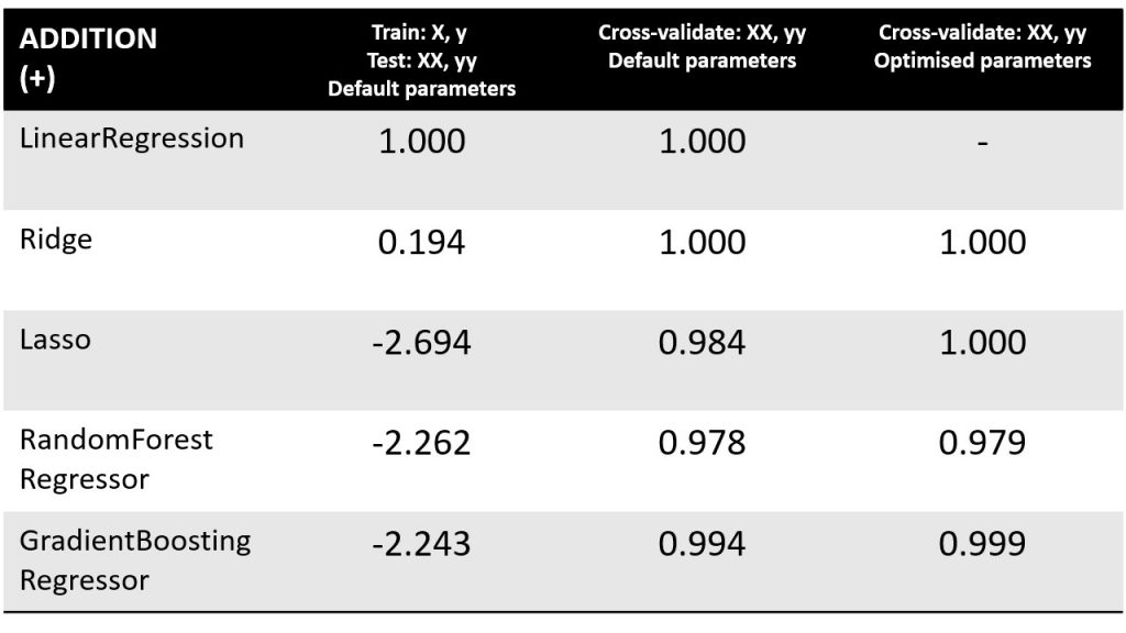
We get output as follows. Test score is max at 1.000, which means every question has been answered correctly:
LinearRegression            test score =  1.000
Ridge                       test score =  0.194
Lasso                       test score = -2.694
RandomForestRegressor       test score = -2.262
GradientBoostingRegressor   test score = -2.243
Test scores <0 means we would do a much better job by taking the average of all the data points we have, and give this average as the answer to any question posed.
The first model, LinearRegression, did a perfect job. After learning from just 3 samples, it is able to solve 100 addition problems correctly! We can in fact take a closer look at the coefficients and intercept found by the linear regressor:
model = LinearRegression()
model.fit(X, y)
print('{:10.3f}{:10.3f}{:10.3f}'.format(model.coef_[0], model.coef_[1], model.intercept_))
We find that both coefficients are one, and the intercept is zero. No magic and no surprise here. m1x1 + m2x2 + c = x1 + x2 when both coefficients m1=1 and m2=1, and intercept c=0. The linear regressor is able to do a perfect job because the 3 points uniquely define the straight line representing the + operation: x1 + x2 = y.
Test scores from the remaining 4 models don’t look good though, but we can’t possibly expect anyone to be able to learn how to add perfectly just by telling him 0+1=1, 1+2=3 and 2+1=3. That isn’t a fair expectation at all. So, let us be more generous with learning materials. From the larger, 100-point dataset we pick 90 data points as learning material, and reserve the remaining 10 data points as test questions. Repeat this procedure 10 times, each time with a different selection of data points (a technique known as cross validation), so that we can get a more representative (less erratic) score:
def cv(model):
     cvscores = cross_validate(model, XX, yy, cv=10, return_train_score=True)
     print('cross_validate test score = {:6.3f}  {:6.3f}  {:6.3f}  {:.0e}'.format(cvscores['test_score'].mean(), cvscores['test_score'].min(), cvscores['test_score'].max(), np.std(cvscores['test_score'])))

def callcvs():
    print('{:28s}'.format('LinearRegression'), end='')
    cv(LinearRegression(n_jobs=-1))
    print('{:28s}'.format('Ridge'), end='')
    cv(Ridge(random_state=rs))
    print('{:28s}'.format('Lasso'), end='')
    cv(Lasso(random_state=rs))
    print('{:28s}'.format('RandomForestRegressor'), end='')
    cv(RandomForestRegressor(n_estimators=100, random_state=rs))
    print('{:28s}'.format('GradientBoostingRegressor'), end='')
    cv(GradientBoostingRegressor(random_state=rs))

callcvs()
We find astounding improvements, so the poor performance we saw earlier was due to insufficient learning materials (training data in machine learning parlance):
LinearRegression            cross_validate test score =  1.000   1.000   1.000  0e+00
Ridge                       cross_validate test score =  1.000   1.000   1.000  3e-07
Lasso                       cross_validate test score =  0.984   0.980   0.987  2e-03
RandomForestRegressor       cross_validate test score =  0.978   0.959   0.992  1e-02
GradientBoostingRegressor   cross_validate test score =  0.994   0.990   0.997  2e-03
So far we have been running all of the above models with default settings (or parameters). Obviously, defaults are not always the best. If we really, really like to push for the best, we can sweep through some pre-defined ranges to find the best parameters:
def gsearchcv(model, param_grid):
     grid_search = GridSearchCV(model, param_grid=param_grid, cv=10, return_train_score=True)
     grid_search.fit(XX, yy)
     print('GridSearch best score = {:6.3f} {}'.format(grid_search.best_score_, grid_search.best_params_))

logrange = np.asarray([.001, .01, .1, 1, 10, 100])
zero2onerange = np.arange(0, 1.1, .1)
neighbourrange = np.arange(25, 300)
lrrange = np.asarray([.00001, .0001, .001, .01, .1])
one2fiverange = np.arange(1, 6)
ten2twothourange = np.arange(50, 1001, 50)

def callgsearchcvs():
    print('{:28s}'.format('Ridge'), end='')
    param_grid = {'alpha': logrange}
    gsearchcv(Ridge(random_state=rs), param_grid)

    print('{:28s}'.format('Lasso'), end='')
    param_grid = {'alpha': logrange, 'max_iter': 1000/logrange}
    gsearchcv(Lasso(random_state=rs), param_grid)

    print('{:28s}'.format('RandomForestRegressor'), end='')
    param_grid = {'n_estimators': neighbourrange}
    gsearchcv(RandomForestRegressor(n_jobs=-1, random_state=rs), param_grid)

    print('{:28s}'.format('GradientBoostingRegressor'), end='')
    param_grid = {'n_estimators':neighbourrange, 'learning_rate': lrrange, 'max_depth': one2fiverange}
    gsearchcv(GradientBoostingRegressor(random_state=rs), param_grid)

callgsearchcvs()
We see some improvements:
Ridge                       GridSearch best score =  1.000 {'alpha': 0.001}
Lasso                       GridSearch best score =  1.000 {'alpha': 0.001, 'max_iter': 1000000.0}
RandomForestRegressor       GridSearch best score =  0.979 {'n_estimators': 193}
GradientBoostingRegressor   GridSearch best score =  0.999 {'learning_rate': 0.1, 'max_depth': 1, 'n_estimators': 299}
Feature importances
We can look at the feature importances found by RandomTreeRegressor before and after optimisation:
before = RandomForestRegressor()
before.fit(XX, yy)
after = RandomForestRegressor(n_estimators=193)
after.fit(XX, yy)
print(before.feature_importances_)
print(after.feature_importances_)
As expected following optimisation, feature importances of m1x1 and m2x2 should be 0.5 and 0.5 i.e. balancely shared half and half, since the two operands are permutable and equally important.
[0.51985616 0.48014384]
[0.50456189 0.49543811]
The following table summarises what we’ve got so far for the addition arithmetic operation. We shall do the same for subtraction, multiplication and division.
Subtract
We can easily repeat what we have done so far, for – (subtraction) instead of + (addition). Some minor modifications to X, Y, XX and YY would do:
X = np.array([[0, 1],
              [1, 2],
              [2, 1]], dtype='int')
y = np.array([-1,
              -1,
               1], dtype='int')

XX = []
for a in range(10):
    for b in range(10):
        XX.append([a, b])
XX = np.asarray(XX, dtype='int')
i = np.arange(len(XX))
np.random.shuffle(i)
XX = XX[i]
yy = np.subtract(XX[:,0], XX[:,1])
We can inspect the data and convince ourselves that each row in the data subtracts correct:
for n in range(5):
     print(XX[n], yy[n])
We get:
[5 0] 5
[8 4] 4
[0 3] -3
[7 3] 4
[6 8] -2
With the new data, we may then re-run the fitscore function:
callfitscores()
We get results similar to what we first got for the + (addition) operation: LinearRegressor scores perfectly (test score = 1.000), while the remaining models score badly:
LinearRegression            test score =  1.000
Ridge                       test score =  0.732
Lasso                       test score = -0.007
RandomForestRegressor       test score =  0.140
GradientBoostingRegressor   test score =  0.133
We can inspect the coefficients and intercept LinearRegressor found:
model = LinearRegression()
model.fit(X, y)
print('{:10.3f}{:10.3f}{:10.3f}'.format(model.coef_[0], model.coef_[1], model.intercept_))
As expected for x1 – x2 = y, the coefficients would now be 1 and -1, while the intercept remains zero.
Next, we re-run the cv function:
callcvs()
and find that given generous training data, models previously found to underperform are now doing much better. As in the case of addition (+), LinearRegression and Ridge score 1.000 while the remaining models score above 0.97:
LinearRegression            cross_validate test score =  1.000   1.000   1.000  0e+00
Ridge                       cross_validate test score =  1.000   1.000   1.000  2e-07
Lasso                       cross_validate test score =  0.983   0.980   0.987  2e-03
RandomForestRegressor       cross_validate test score =  0.978   0.954   0.997  1e-02
GradientBoostingRegressor   cross_validate test score =  0.993   0.980   0.998  5e-03
That cross-validation was done with default parameter settings of each model. Next, let us do it with optimised parameters:
callgsearchcvs()
We see some improvements as follows:
Ridge                       GridSearch best score =  1.000 {'alpha': 0.001}
Lasso                       GridSearch best score =  1.000 {'alpha': 0.001, 'max_iter': 1000000.0}
RandomForestRegressor       GridSearch best score =  0.981 {'n_estimators': 149}
GradientBoostingRegressor   GridSearch best score =  1.000 {'learning_rate': 0.1, 'max_depth': 1, 'n_estimators': 299}
Table 2 summarises what we’ve got for the subtraction operation.

Multiply
We can easily repeat what we have done so far, for × (multiplication) instead of + (addition) and – (subtraction). We redefine X, Y, XX and YY:
X = np.array([[0, 1],
              [1, 2],
              [2, 1]], dtype='int')
y = np.array([0,
              2,
              2], dtype='int')

XX = []
for a in range(10):
    for b in range(10):
        XX.append([a, b])
XX = np.asarray(XX, dtype='int')
i = np.arange(len(XX))
np.random.shuffle(i)
XX = XX[i]
yy = np.multiply(XX[:,0], XX[:,1])
We can inspect the data and convince ourselves that each row in the data adds up correct:
for n in range(5):
     print(XX[n], yy[n])
We find:
[8 5] 40
[9 3] 27
[1 1] 1
[1 0] 0
[9 2] 18
We may then re-run the fitscore function:
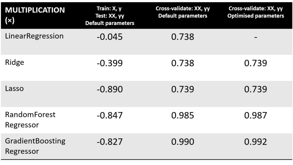
callfitscores()
This time, all models do badly. The LinearRegression model, which scored full marks for addition and subtraction, is now failing. The problem is no longer linear.
LinearRegression            test score = -0.045
Ridge                       test score = -0.399
Lasso                       test score = -0.890
RandomForestRegressor       test score = -0.847
GradientBoostingRegressor   test score = -0.827
Next, we re-run the cv function, which is more generous with training data:
callcvs()
We get:
LinearRegression            cross_validate test score =  0.738   0.264   0.909  2e-01
Ridge                       cross_validate test score =  0.738   0.265   0.909  2e-01
Lasso                       cross_validate test score =  0.739   0.272   0.902  2e-01
RandomForestRegressor       cross_validate test score =  0.985   0.969   0.997  9e-03
GradientBoostingRegressor   cross_validate test score =  0.990   0.978   0.997  7e-03
Ensemble trees (RandomForestRegressor and GradientBoosting Regressor) now beat the linear models (LinearRegression, Ridge and Lasso)! That’s because the problem is no longer linear. We can optimise the parameters by calling our function callgsearchcvs:
callgsearchcvs()
We get the output:
Ridge                       GridSearch best score =  0.739 {'alpha': 10.0}
Lasso                       GridSearch best score =  0.739 {'alpha': 1.0, 'max_iter': 1000000.0}
RandomForestRegressor       GridSearch best score =  0.987 {'n_estimators': 145}
GradientBoostingRegressor   GridSearch best score =  0.992 {'learning_rate': 0.1, 'max_depth': 3, 'n_estimators': 298}
The problem is clearly beyond the linear models (Ridge and Lasso). Ensemble trees (random forest and gradient boosting) are able to get their division right >98% of the time. Table 3 summarises what we’ve got for the multiplication operation.
Divide
We can easily repeat what we have done so far, for ÷ (divide) instead. In addition to redefining X, Y, XX and YY, we also need to be careful not to create data points which cause divisions by zero:
X = np.array([[0, 1],
              [1, 2],
              [2, 1]], dtype='int')
y = np.array([0,
              .5,
              2])

XX = []
for a in range(10):
    for b in range(10):
        XX.append([a, b])
XX = np.asarray(XX, dtype='int')
XX = XX[XX[:,1]>0]
i = np.arange(len(XX))
np.random.shuffle(i)
XX = XX[i]
yy = np.divide(XX[:,0], XX[:,1])
We can inspect the data and convince ourselves that each row in the data adds up correct:
for n in range(5):
     print(XX[n], yy[n])
We get:
[8 6] 1.3333333333333333
[9 6] 1.5
[3 9] 0.3333333333333333
[7 3] 2.3333333333333335
[6 4] 1.5
We may then re-run the fitscore function:
callfitscores()
The results would be similar to the multiplication case. All models, including LinearRegression, do badly:
LinearRegression            test score = -1.160
Ridge                       test score = -0.169
Lasso                       test score = -0.117
RandomForestRegressor       test score =  0.154
GradientBoostingRegressor   test score =  0.113
Next, we re-run the cv function, which is more generous with training data:
callcvs()
We get something like:
LinearRegression            cross_validate test score =  0.209  -2.955   0.788  1e+00
Ridge                       cross_validate test score =  0.212  -2.933   0.789  1e+00
Lasso                       cross_validate test score =  0.421  -0.673   0.749  4e-01
RandomForestRegressor       cross_validate test score =  0.945   0.786   0.989  6e-02
GradientBoostingRegressor   cross_validate test score =  0.961   0.923   0.997  3e-02
Once again, ensemble trees (RandomForestRegressor and GradientBoosting Regressor) beat the linear models (LinearRegression, Ridge and Lasso)! As in the case for multiplication between two numbers, division of one number by another is not a linear problem.
We can optimise the parameters by calling our function callgsearchcvs:
callgsearchcvs()
We get the output:
Ridge                       GridSearch best score =  0.393 {'alpha': 100.0}
Lasso                       GridSearch best score =  0.421 {'alpha': 1.0, 'max_iter': 1000000.0}
RandomForestRegressor       GridSearch best score =  0.953 {'n_estimators': 41}
GradientBoostingRegressor   GridSearch best score =  0.964 {'learning_rate': 0.1, 'max_depth': 3, 'n_estimators': 299}
As expected, the problem is beyond the linear models (Ridge and Lasso). Ensemble trees (random forest and gradient boosting) are able to get their division right >93% of the time. Table 4 summarises what we’ve got for the division operation.

If GradientBoostingRegressor is able to divide correctly 95% of the time, we start wondering what happens to the balance 5%. When it divides wrongly, how far does it go wrong? Let’s take a closer look:
model = GradientBoostingRegressor(learning_rate=.1, max_depth=4, n_estimators=299, random_state=rs)
model.fit(XX, yy)
p = model.predict(XX)
d = np.subtract(p, yy)
%matplotlib inline
import matplotlib.pyplot as plt
plt.hist(d, 20)
plt.savefig('gbr_subtract.png')

We find that the maximum difference from the correct answer is 0.03 (Figure 1), so GradientBoostingRegressor does manage to get all answers correct to the third significant figure, which isn’t that bad.
Add, subtract, multiply and divide
Up till now we’ve been getting the machine to learn to either add, subtract, multiply or divide. We provided the machine with add-only data, and tested its performance on adding. We then trained the machine with subtract-only data, then tested how well it was able to subtract. We followed with similar isolated train-test experiments for multiplication and division.
What if we’d like our trained machine to be able to do all 4 arithmetic operations (add, subtract, multiply and divide) within the same train-test exercise? This is what we are going to do next.
We shall redefine X, Y, XX and YY to include data for all 4 arithmetic operations. In addition, we will add a third feature to each data point. This third feature will carry the information as to whether that data point is for addition, subtraction, multiplication or division. Here, I use 0 to represent +, 1 to represent -, 2 to represent × and 3 to represent ÷. Like this:
X = np.array([[0, 0, 0],
              [1, 2, 0],
              [2, 1, 0],
              [0, 0, 1],
              [1, 2, 1],
              [2, 1, 1],
              [0, 0, 2],
              [1, 2, 2],
              [2, 1, 2],
              [0, 1, 3],
              [1, 2, 3],
              [2, 1, 3]], dtype='int')
y = np.array([0,
              3,
              3,
              0,
             -1,
              1,
              0,
              2,
              2,
              0,
              .5,
              2])

XX = []
for a in range(10):
    for b in range(10):
        XX.append([a, b, 0])
XX = np.asarray(XX, dtype='int')
yy_add = np.add(XX[:,0], XX[:,1])
yy_sub = np.subtract(XX[:,0], XX[:,1])
yy_mul = np.multiply(XX[:,0], XX[:,1])
XX_div = XX[XX[:,1]>0]
yy_div = np.divide(XX_div[:,0], XX_div[:,1])
XX = np.concatenate((XX, XX, XX, XX_div))
XX[100:, 2] = 1
XX[200:, 2] = 2
XX[300:, 2] = 3
yy = np.concatenate((yy_add, yy_sub, yy_mul, yy_div))
i = np.arange(len(XX))
np.random.shuffle(i)
XX = XX[i]
yy = yy[i]
We can inspect the data and convince ourselves that for each row in the data, where the 3rd column of XX is 0, the features add up correctly. And where the 3rd column of XX is 1, the 2nd feature is subtracted from the first correctly. And where the 3rd column of XX is 2, the product of the features is correct. And where the 3rd column of XX is 3, the first feature gets divided by the second correctly.
for n in range(5):
     print(XX[n], yy[n])
We get:
[0 3 0] 3.0
[5 3 2] 15.0
[5 5 3] 1.0
[4 3 1] 1.0
[9 7 0] 16.0
Now, X and Y each contain 12 data points rather than 3. The first 3 data points are for addition, the next 3 for subtraction, followed by another 3 for multiplication and another 3 for division. Likewise, XX and YY now contain 3 features (columns) for each data point (row). All 4 arithmetic operations are now included in XX and YY. With these data in hand, we call our fitscore, cv and gsearchcv functions the same way as we did.
callfitscores()
We get:
LinearRegression            test score =  0.074
Ridge                       test score =  0.056
Lasso                       test score = -0.260
RandomForestRegressor       test score = -0.184
GradientBoostingRegressor   test score = -0.128
Next, we call:
callcvs()
and we get:
LinearRegression            cross_validate test score =  0.061  -0.723   0.227  3e-01
Ridge                       cross_validate test score =  0.061  -0.722   0.227  3e-01
Lasso                       cross_validate test score =  0.072  -0.637   0.213  2e-01
RandomForestRegressor       cross_validate test score =  0.988   0.979   0.996  5e-03
GradientBoostingRegressor   cross_validate test score =  0.875   0.778   0.960  6e-02
And then we call:
callgsearchcvs()
and we find that ensemble trees are still able to get >99% of the answers correct:
Ridge                       GridSearch best score =  0.066 {'alpha': 100.0}
Lasso                       GridSearch best score =  0.072 {'alpha': 1.0, 'max_iter': 1000000.0}
RandomForestRegressor       GridSearch best score =  0.990 {'n_estimators': 116}
GradientBoostingRegressor   GridSearch best score =  0.992 {'learning_rate': 0.1, 'max_depth': 5, 'n_estimators': 297}
Table 5 summarises the test scores.

So far so good. We experimented with:
- linear (addition and subtraction) as well as nonlinear problems (multiplication and division);
- linear models (linear regression, Ridge and Lasso) as well as ensemble trees (random forest and gradient boosting);
- training and testing on separate datasets, as well as training and testing by cross-validation;
- training models with default as well as parameters optimised using scikit-learn’s GridSearchCV.