Jupyter notebook for this exercise can be downloaded here:
We are frequently exposed to the loose nomenclature interchanging grayscale and black-and-white. Grayscale images are not black-and-white. Grayscales contain different shades of gray and allow a range of pixel values. Black-and-white images contain only 2 pixel vales; nothing in between.
In the MNIST problem, handwritten digits are provided in the form of grayscale images. I don’t think we need grayscale images. I don’t think the different shades of gray offers any additional information as to which digit the image shows. The shades of gray originate from how strong the writer writes, and perhaps some inconsistencies from the pen too. Neither tells us any extra information on which digit the handwritting represents.
We shall test it out here.
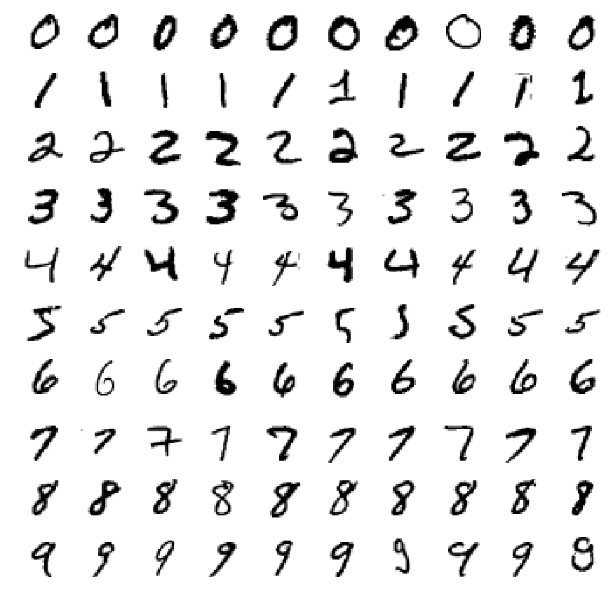
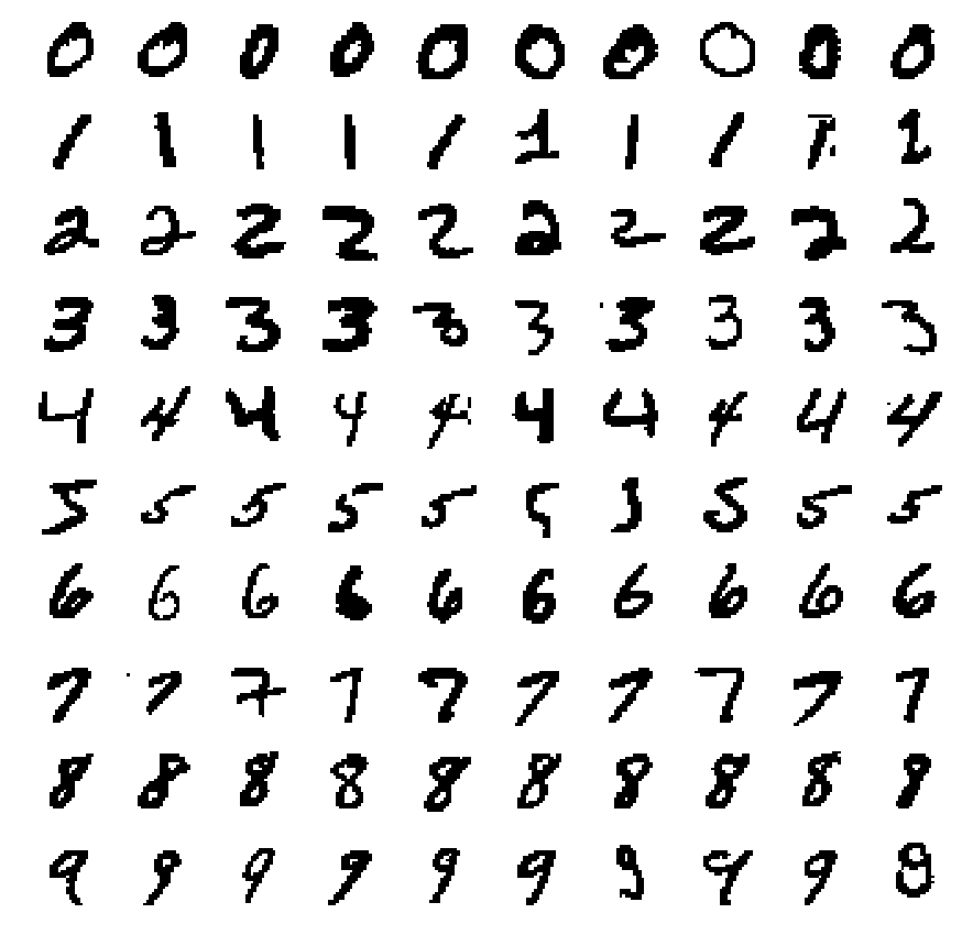
Let us convert the original grayscale images of MNIST to black-and-white. The original grayscale ranged from 0 to 255. Taking 125 as threshold, we turn all pixels <125 to zero, and turn all other pixels to 1:
from keras.datasets import mnist
from keras.utils import to_categorical
from keras import models, layers, callbacks
import time
import numpy as np
np.random.seed(77)

(train_X, train_y), (test_X, test_y) = mnist.load_data()
nclasses = np.unique(train_y).size
threshold = 125
def shapex(X):
    XX = np.empty_like(X)
    XX[X< threshold] = 0
    XX[X>=threshold] = 1
    XX = XX.reshape(*XX.shape, 1)
    return XX
train_X = shapex(train_X)
test_X = shapex(test_X)
train_y = to_categorical(train_y)
test_y = to_categorical(test_y)
My version of model.summary():
def summarisetis(model):
     s = '{}'.format(model.optimizer).split(' ')[0].split('.')[-1]
     print(s)
     print('{:12s}{:>10s}{:>10s}{:>10s}{:>10s}{:>10s}{:>10s}'.format('class', 'input', 'output', 'units', 'params', 'activ', 'label'))
     print('========================================================================')
     modellabel = s + ':'
     for nl, l in enumerate(model.layers):
         s = '{}'.format(l).split(' ')[0].split('.')[-1]
         print('{:12s}{:10d}'.format(s,l.input_shape[1]), end='')
         print('{:10d}'.format(l.output_shape[1]), end='')
         layerlabel = s[:2]
         try:
             layerlabel = f'{layerlabel}{l.units}'
             print('{:10d}'.format(l.units), end='')
         except:
             print('{:10s}'.format(''), end='')
         print('{:10d}'.format(l.count_params()), end='')
         try:
             s = '{}'.format(l.activation).split(' ')[1]
             layerlabel = layerlabel + s[:3]
             print('{:>10s}{:>10s}'.format(s, layerlabel))
         except:
             print('{:10s}{:>10s}'.format('', layerlabel))
         modellabel = modellabel + layerlabel
         if nl < len(model.layers)-1:
             modellabel = modellabel + '|'
     print('labelling this model as', modellabel,'\n')
     return modellabel
We use the same architecture (with Conv2D) as previously done:
def arch():
     m = models.Sequential()
     m.add(layers.Conv2D(32, (3,3), activation='relu', input_shape=train_X.shape[1:]))
     m.add(layers.MaxPooling2D((2,2)))
     m.add(layers.Conv2D(64, (3,3), activation='relu'))
     m.add(layers.MaxPooling2D((2,2)))
     m.add(layers.Conv2D(64, (3,3), activation='relu'))
     m.add(layers.Flatten())
     m.add(layers.Dense(64, activation='relu'))
     m.add(layers.Dense(nclasses, activation='softmax'))
     return m

def compiletis(model, op):
     model.compile(optimizer=op,
                       loss='categorical_crossentropy',
                    metrics=['accuracy'])
     return model
For plotting:
%matplotlib inline
import matplotlib.pyplot as plt
def plottis(history):
     acc = history.history['acc']
     val_acc = history.history['val_acc']
     loss = history.history['loss']
     val_loss = history.history['val_loss']

     plt.figure(figsize=(10, 3))
     plt.subplot(121)
     plt.plot(range(1, len(loss) + 1), loss, label='training')
     plt.plot(range(1, len(val_loss) + 1), val_loss, label='validation')
     plt.xlabel('epoch')
     plt.ylabel('loss')

     plt.subplot(122)
     plt.plot(range(1, len(acc) + 1), acc, label='training')
     plt.plot(range(1, len(val_acc) + 1), val_acc, label='validation')
     plt.xlabel('epoch')
     plt.ylabel('accuracy')
Fit with callback:
cb = callbacks.EarlyStopping(monitor='val_loss',
                              min_delta=0,
                              patience=5,
                              verbose=0, mode='auto')
def fittis(model, bs, ep):
     tic = time.perf_counter()
     history = model.fit(train_X, train_y,
                         epochs=ep, batch_size=bs,
                         validation_split=.3, verbose=0,
                         callbacks = [cb])
     plottis(history)
     train_acc = history.history['acc']
     train_los = history.history['loss']
     val_acc   = history.history['val_acc']
     val_los   = history.history['val_loss']
     iacc = 1+int(min(np.where(val_acc==max(val_acc))[0]))
     ilos = 1+int(min(np.where(val_los==min(val_los))[0]))
     model.fit(train_X, train_y, epochs=ilos, batch_size=bs, verbose=0)
     _, test_acc = model.evaluate(test_X, test_y)
     tim = time.perf_counter()-tic
     print('train_acc = {:.3f}    val_acc = {:.3f}    epochs = {:3d}    test_acc = {:.3f}    time = {:.1e}'.format
           (max(train_acc), max(val_acc), ilos, test_acc, tim))
     myhistory = [train_acc, train_los, val_acc, val_los, iacc, ilos, test_acc, tim]
     return model, myhistory

myhistory = []
model = compiletis(arch(), 'rmsprop')
summarisetis(model)
s = '{}'.format(model.layers[0])
model, h = fittis(model, bs=4096, ep=100)
myhistory.append(h)
We get:
RMSprop
class            input    output     units    params     activ     label
========================================================================
Conv2D              28        26                 320      relu     Corel
MaxPooling2D        26        13                   0                  Ma
Conv2D              13        11               18496      relu     Corel
MaxPooling2D        11         5                   0                  Ma
Conv2D               5         3               36928      relu     Corel
Flatten              3       576                   0                  Fl
Dense              576        64        64     36928      relu   De64rel
Dense               64        10        10       650   softmax   De10sof
labelling this model as RMSprop:Corel|Ma|Corel|Ma|Corel|Fl|De64rel|De10sof
10000/10000 [==============================] - 1s 53us/step
train_acc = 0.997    val_acc = 0.987    epochs =  45    test_acc = 0.991    time = 3.9e+01
Compared to our previous training using original grayscale MNIST images, a test_acc of 0.991 isn’t bad at all! Results support my argument that grayscales add no additional information to digit differentiation.