Neural networks with Keras

The Jupyter notebook for this exercise can be downloaded here.

%matplotlib inline
import matplotlib.pyplot as plt
import keras.backend as K 
from keras import models, layers, optimizers
from sklearn.preprocessing import StandardScaler
import time
import numpy as np
np.random.seed(77)

X = []
samplesize = 1e5
for a in range(int(samplesize**.5)):
     for b in range(1, int(samplesize**.5)):
         X.append([a, b, a+b, 1, 0, 0, 0])
         X.append([a, b, a-b, 0, 1, 0, 0])
         X.append([a, b, a*b, 0, 0, 1, 0])
         X.append([a, b, a/b, 0, 0, 0, 1])
X = np.asarray(X)
np.random.shuffle(X)
X[:, :3] = StandardScaler().fit_transform(X[:, :3])
y = X[:, 2]
X = np.delete(X, 2, 1)

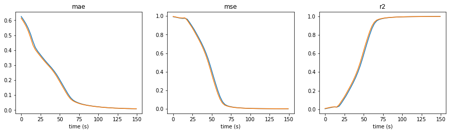
def plottis(history, tim):
    plt.figure(figsize=(15, 8))
    t = np.linspace(0, tim, len(history['loss']))
    plt.subplot(231)
    plt.plot(t, history['loss']); plt.title('mae')
    plt.plot(t, history['val_loss']); plt.xlabel('time (s)')
    plt.subplot(232)
    plt.plot(t, history['mean_squared_error']); plt.title('mse')
    plt.plot(t, history['val_mean_squared_error']); plt.xlabel('time (s)')
    plt.subplot(233)
    plt.plot(t, history['r2']); plt.title('r2'); 
    plt.plot(t, history['val_r2']); plt.xlabel('time (s)')

def fittis(hu, ly, lr, bs):
    def r2(y_true, y_pred):
        SS_res =  K.sum(K.square( y_true-y_pred ))
        SS_tot = K.sum(K.square( y_true - K.mean(y_true) ) )
        return ( 1 - SS_res/(SS_tot + K.epsilon()) )   
    tic = time.perf_counter()
    model = models.Sequential()
    model.add(layers.Dense(hu, activation='relu', input_shape=(X.shape[1],)))
    for _ in range(ly-1):
        model.add(layers.Dense(hu, activation='relu'))
    model.add(layers.Dense(1))
    model.compile(optimizer=optimizers.RMSprop(lr=lr),
                  loss='mae',
                  metrics=['mse', r2])
    history = model.fit(X, y, 
                        epochs=50, batch_size=bs,
                        validation_split=.2, verbose=1)
    tim = time.perf_counter()-tic
    plottis(history.history, tim)
    train_los = history.history['loss']
    train_mse = history.history['mean_squared_error']
    train_r2  = history.history['r2']
    val_los   = history.history['val_loss']
    val_mse   = history.history['val_mean_squared_error']
    val_r2    = history.history['val_r2']
    return model, history

bs = 1024
hu = 20
ly = 10
lr = 1e-5
m, h = fittis(hu, ly, lr, bs)

Epoch 50/50
318528/318528 [==============================] - 3s 8us/step - loss: 0.0091 - mean_squared_error: 5.3479e-04 - r2: 0.9995 - val_loss: 0.0092 - val_mean_squared_error: 5.7709e-04 - val_r2: 0.9994