Category Encoders: Catalog & Experiments (Part 2)
We get 24 encoders from 4 libraries:
| library | one-hot encoders | other simple encoders | contrast encoders | target/Bayesian encoders |
|---|---|---|---|---|
| sklearn | OneHotEncoder | LabelEncoder OrdinalEncoder LabelBinarizer | ||
| category_encoders | OneHotEncoder | OrdinalEncoder BinaryEncoder BaseNEncoder CountEncoder HashingEncoder | HelmertEncoder SumEncoder BackwardDifferenceEncoder PolynomialEncoder | TargetEncoder LeaveOneOutEncoder CatBoostEncoder MEstimateEncoder WOEEncoder JamesSteinEncoder GLMMEncoder |
| pandas | get_dummies | factorize | ||
| keras.utils | to_categorical |
This notebook explores step-by-step the Hashing Encoder, the Polynomial Encoder and some flavours/variations of the target encoder. All flavours of target encoders peeks into the target; we therefore need to be mindful of data leakage. Options are available to regulate/control data leakage and overfitting. TargetEncoder is the vanilla flavour. LeaveOneOutEncoder is the conservative option, where a given sample sees other samples’ target but blindfolded from it’s own. CatBoostEncoder is sensitive to row ordering; a given sample sees the target of preceding samples only. JamesSteinEncoder is for normal distributions.
In particular, we have in this notebook
TargetEncoder(the vanilla form) demonstrated in detail to tell the principle behind target encoding, which underlies all flavours of target encoding. Manual back-of-envelop derivation is compared with automated output fromTargetEncoder.LeaveOneOutEncoderdemonstrated in detail as a conservative step up to reduce data leakage and overfitting. Manual back-of-envelop derivation is compared with automated output fromLeaveOneOutEncoder.
This notebook continues from an earlier notebook, Category Encoders: Catalog & Experiments (Part 1).
When to use which encoder to solve what problems? There is a good guide here: [Encode Smarter: How to Easily Integrate Categorical Encoding into Your Machine Learning Pipeline](https://innovation.alteryx.com/encode-smarter).
from sklearn.preprocessing import LabelEncoder
from category_encoders import HashingEncoder, PolynomialEncoder
from category_encoders import TargetEncoder, LeaveOneOutEncoder, MEstimateEncoder, WOEEncoder, JamesSteinEncoder, CatBoostEncoder, GLMMEncoder
from keras import utils

import numpy as np
import pandas as pd
import matplotlib.pyplot as plt
import warnings, gc, time
warnings.simplefilter('ignore') # once | error | always | default | module

from tqdm import tqdm_notebook

# We shall be compiling a summary table as we go along.
summary = pd.DataFrame({'inp2out_map': pd.Series(dtype=object),   # input-to-output map
                        'nunique'    : pd.Series(dtype=int),      # number of unique (or distinct) values in output
                        'unique'     : pd.Series(dtype='object'), # unique values in output
                        'shape'      : pd.Series(dtype=int),      # rows-by-columns of output array
                        'tictoc'     : pd.Series(dtype=int)})     # computation time i seconds
summary.index.name = 'encoder'
# The grand summary is printed at the end of this notebook.
train = pd.read_csv('/kaggle/input/tabular-playground-series-mar-2021/train.csv', index_col='id')
train.sample(5)# Let's zoom into a single column.
train['cat10'].nunique(), train['cat10'].unique()
# cat10 alone has 299 unique values altogether. This value in termed 'cardinality'.
# This is an extreme case. Cardinalities are usually lower e.g. exam grades = A, B, C, D, E would have cardinality=5.(299,
array(['LO', 'HJ', 'DJ', 'KV', 'DP', 'GE', 'HQ', 'HC', 'EK', 'GS', 'HG',
'BY', 'HX', 'JK', 'FJ', 'LM', 'HK', 'MD', 'IG', 'JG', 'AN', 'AD',
'MC', 'KW', 'CK', 'LF', 'CS', 'GK', 'DC', 'LB', 'FM', 'IH', 'LN',
'IK', 'DF', 'IB', 'CB', 'LY', 'JW', 'FI', 'CR', 'IE', 'LE', 'HB',
'HV', 'LG', 'BG', 'KP', 'LI', 'HL', 'BF', 'LU', 'O', 'GI', 'DQ',
'IR', 'DV', 'HA', 'KB', 'FP', 'AT', 'IF', 'HN', 'GC', 'C', 'KC',
'G', 'JA', 'CU', 'BC', 'AB', 'KF', 'MB', 'HE', 'BL', 'FQ', 'IA',
'MJ', 'FO', 'V', 'JT', 'AU', 'IO', 'GQ', 'CC', 'JR', 'BM', 'HH',
'AV', 'GT', 'I', 'IU', 'JN', 'EV', 'MV', 'EQ', 'LW', 'FN', 'IT',
'AA', 'DK', 'IJ', 'GU', 'P', 'JH', 'CM', 'GA', 'R', 'LX', 'IX',
'DY', 'D', 'FL', 'CP', 'GL', 'DI', 'CD', 'IV', 'FS', 'FR', 'J',
'MP', 'MH', 'EL', 'JD', 'AP', 'AE', 'F', 'LC', 'BP', 'BI', 'MF',
'DO', 'MG', 'MT', 'LD', 'CW', 'KS', 'BV', 'JV', 'BB', 'AM', 'KX',
'FK', 'AH', 'LV', 'W', 'DU', 'FB', 'JX', 'KA', 'CO', 'AR', 'KR',
'JI', 'T', 'JP', 'LQ', 'FX', 'FD', 'EY', 'Y', 'JO', 'EC', 'HM',
'AC', 'DW', 'HU', 'FH', 'AY', 'AL', 'GD', 'GB', 'DS', 'FT', 'KH',
'CG', 'JB', 'E', 'CN', 'BT', 'X', 'BX', 'HW', 'EI', 'ID', 'KT',
'GR', 'L', 'KG', 'EA', 'HO', 'GX', 'K', 'AS', 'DM', 'AK', 'FC',
'MS', 'HR', 'EU', 'ES', 'JY', 'HP', 'KL', 'FE', 'CY', 'EO', 'KJ',
'CJ', 'CI', 'JL', 'IC', 'S', 'DH', 'GN', 'BS', 'AG', 'M', 'EW',
'FA', 'LJ', 'GJ', 'KQ', 'HF', 'MR', 'BQ', 'ED', 'FG', 'LL', 'EG',
'HY', 'EH', 'GW', 'BD', 'IQ', 'Q', 'DA', 'DD', 'GM', 'KN', 'MQ',
'GY', 'KD', 'JJ', 'CL', 'IY', 'KU', 'CT', 'KK', 'DN', 'BO', 'IP',
'LH', 'IM', 'DE', 'ME', 'EE', 'LT', 'LR', 'MI', 'CF', 'DR', 'EB',
'KI', 'DX', 'DL', 'MW', 'FF', 'EF', 'EP', 'MU', 'MA', 'GG', 'CQ',
'DT', 'FV', 'CH', 'AF', 'AJ', 'IN', 'JC', 'EN', 'JU', 'JE', 'ML',
'AW', 'HI', 'MO', 'GF', 'MK', 'GH', 'FW', 'GV', 'JF', 'BA', 'LK',
'IL', 'CX'], dtype=object))# Now pick another column; just to have a look.
train['cat5'].nunique(), train['cat5'].unique()
# Lower cardinality in this column; 84 only.(84,
array(['BI', 'AB', 'BU', 'M', 'T', 'K', 'L', 'CG', 'BG', 'CI', 'N', 'G',
'X', 'Q', 'O', 'BO', 'BB', 'BX', 'AF', 'BA', 'BQ', 'CA', 'D', 'AQ',
'AS', 'AW', 'BE', 'CK', 'AL', 'BK', 'AT', 'CL', 'C', 'CF', 'I',
'AH', 'CD', 'AY', 'BY', 'F', 'AI', 'R', 'BC', 'BH', 'AA', 'V',
'CE', 'BD', 'AE', 'U', 'AU', 'AP', 'CJ', 'AN', 'AX', 'AR', 'BL',
'J', 'ZZ', 'BR', 'BV', 'H', 'A', 'CC', 'P', 'CH', 'BJ', 'CB', 'BS',
'BN', 'AO', 'AJ', 'BT', 'S', 'E', 'Y', 'AK', 'AM', 'B', 'BM', 'AV',
'AG', 'BF', 'BP'], dtype=object))1. Hashing Encoder
What is a Hashing Encoder? The question becomes immediately self-explanatory the moment we read the word hashing in the light of MD5, SHA, .... Yes, it’s that same hash that the hashing encoder is about.
HashingEncoder takes n_components as an argument. Let us do a test with n_components= 8, 16, 32:
%%time
for n_components in [8, 16, 32]:
    inp = train['cat10']
    tic = time.time()
    out = HashingEncoder(n_components=n_components).fit_transform(inp)
    tictoc = time.time() - tic

    inp2out_map = pd.concat([pd.DataFrame({'inp': train['cat10']}, columns=['inp']),
                             pd.DataFrame(out, index=train.index)], axis=1).drop_duplicates()
    inp2out_map.set_index('inp', inplace=True, drop=True)
    unik = np.unique(inp2out_map.values)
    summary.loc[f'HashingEncoder, {n_components}'] = inp2out_map, len(unik), unik, inp2out_map.shape, tictoc
columns_show = ['nunique', 'unique', 'shape', 'tictoc']
summary[columns_show]
# We find that no matter what n_components we asked for, the mapped values always consist of 0 and 1, and nothing else.
# When we ask for n_components=8, we get 8 columns in the output. When we ask for n_components=16, we get 16 columns. When we ask for n_components=32, we get 32 columns.
CPU times: user 932 ms, sys: 1.2 s, total: 2.13 s
Wall time: 6min 56s
summary.loc['HashingEncoder, 8', 'inp2out_map']
# Some rows in inp2out_map contain null values.
# This shows that some categories in the original input (train['cat10']) are not mapped to anything.
# HashingEncoder therefore doesn't map one-to-one i.e. some of the original info is lost in the encoding process.# Now we filter out the null rows and show only non-null rows.
non_null_idx = ~summary.loc['HashingEncoder, 8', 'inp2out_map'].isnull().any(axis=1)
non_null_rows = summary.loc['HashingEncoder, 8', 'inp2out_map'].loc[non_null_idx]
non_null_rows# Next, we see if there are any duplicate rows that can be removed.
non_null_rows.drop_duplicates()
# We are left with just 8 rows! That means many input categories got mapped to the same output value. This loss of info is called *collision*.# Let's repeat what we did in the previous two cells for ```n_components``` = 8, 16, 32:
print('{:15s}{}'.format('n_components', 'unique values of output'))
for n_components in [8, 16, 32]:
non_null_idx = ~summary.loc[f'HashingEncoder, {n_components}', 'inp2out_map'].isnull().any(axis=1)
non_null_rows = summary.loc[f'HashingEncoder, {n_components}', 'inp2out_map'].loc[non_null_idx]
print('{:<15d}{}'.format(n_components, len(non_null_rows.drop_duplicates())))
# The lower number of unique values of output, the higher the collisions i.e. we suffer a greater info loss.n_components unique values of output
8 8
16 16
32 32
2. Polynomial encoder
inp = train['cat5']
tic = time.time()
out = PolynomialEncoder().fit_transform(inp)
tictoc = time.time() - tic

inp2out_map = pd.concat([pd.DataFrame({'inp': train['cat5']}, columns=['inp']),
                         pd.DataFrame(out, index=train.index)], axis=1).drop_duplicates()
inp2out_map.set_index('inp', inplace=True, drop=True)
unik = np.unique(inp2out_map.values)
summary.loc['PolynomialEncoder'] = inp2out_map, len(unik), unik, inp2out_map.shape, tictoc
summary.loc['PolynomialEncoder', 'inp2out_map']
# As shown in [Part 1](https://www.kaggle.com/marychin/category-encoders-catalog-experiments-part-1) of this notebook series, contrast encoders output an ```intercept``` column.# Now we filter out the null rows and show only non-null rows.
non_null_idx = ~summary.loc['PolynomialEncoder', 'inp2out_map'].isnull().any(axis=1)
non_null_rows = summary.loc['PolynomialEncoder', 'inp2out_map'].loc[non_null_idx]
non_null_rows# Next, we see if there are any duplicate rows that can be removed.
non_null_rows.drop_duplicates()
# We get 84 rows still. No collision in this case (unlike HashingEncoder).3. Target Encoders
feature = 'cat5'
for which in [TargetEncoder, LeaveOneOutEncoder, MEstimateEncoder, WOEEncoder, JamesSteinEncoder, GLMMEncoder, CatBoostEncoder]:
#   Grab the label, apply some minor hiding cosmetics:
    label = str(which).split('.')[-1].split("'")[0]

    tic = time.time()
    out = which().fit_transform(train[feature], train['target'])
    tictoc = time.time() - tic
    inp2out_map = pd.concat([pd.DataFrame({'inp': train[feature]}, columns=['inp']),
                             pd.DataFrame(out, index=train.index)], axis=1).drop_duplicates()
    inp2out_map.set_index('inp', inplace=True, drop=True)
    unik = np.unique(inp2out_map.values)
    summary.loc[label] = inp2out_map, len(unik), unik, inp2out_map.shape, tictoc

#   Test if encoding depends on the order of rows.
    shuffled = train[[feature, 'target']].copy()
    shuffled = shuffled.sample(frac=1)
    out_shuffled = which().fit_transform(shuffled[feature], shuffled['target'])
    out.rename(columns={feature: 'tis'}, inplace=True)
    out_shuffled.rename(columns={feature: 'tat'}, inplace=True)
    tistat = pd.concat([out, out_shuffled], names=['tis', 'tat'], axis=1)
    if not np.allclose(tistat['tis'], tistat['tat']):
        print(label, 'is order-dependent.')
columns_show = ['nunique', 'unique', 'shape', 'tictoc']
summary[columns_show]
# Output reports that GLMMEncoder and CatBoostEncoder depend on the order of rows.
GLMMEncoder is order-dependent.
CatBoostEncoder is order-dependent.
3.1 Target Encoder (vanilla)
ncoda = LabelEncoder()
x = ncoda.fit_transform(train['cat5'])
y = train['target']
z = TargetEncoder().fit_transform(train['cat5'], train['target'])

fig = plt.figure(figsize=(15, 15))
ax = fig.add_subplot(projection='3d')
ax.scatter3D(x, y, z, c=z, cmap='hot')
ax.set_xlabel('cat 5'); ax.set_ylabel('target'); ax.set_zlabel(label)
_ = ax.set_xticks(np.arange(0, len(ncoda.classes_), 5))
_ = ax.set_xticklabels(ncoda.classes_[::5])
# 3D plot shows how encoders output depends on both cat5 and target.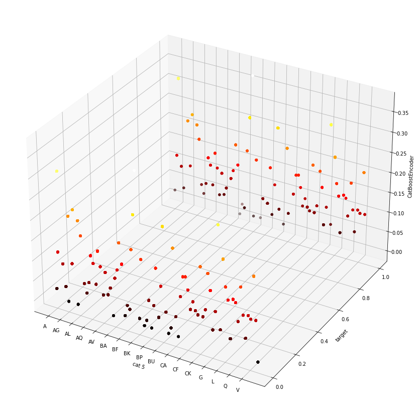
# How does TargetEncoder encode? It takes the mean of the target of the given category.
# Let's have a goal doing this manually, then compare with TargetEncoder's output.
manual_auto = pd.DataFrame( {'manual': train.groupby('cat5')['target'].mean()} )
manual_auto = pd.concat([manual_auto, summary.loc['TargetEncoder', 'inp2out_map']], axis=1)
np.allclose(manual_auto['manual'], manual_auto['cat5'], atol=1e-7)
# So it is confirmed that our manual back-of-envelop calculation agrees with the output by TargetEncoder.True3.2 Leave-One-Out Encoder
LeaveOneOutEncoder is the conservative step up from the vanilla TargetEncoder. It reduces data leakage and overfitting by taking the target mean from rows other than a given row. A worked back-of-envelop example would explain best:
# train contains too many rows. To avoid prohibitive runtimes let's reduce train to a manageable subset.
reduced = train.sample(10000, random_state=77).reset_index(drop=True)

# Now let us try encoding leave-one-out manually.
manual = pd.Series()
for grp_idx, grp_data in tqdm_notebook(reduced.groupby('cat5'), total=reduced['cat5'].nunique()):
    for row_idx, row_data in grp_data.iterrows():
        manual.loc[row_idx] = grp_data.drop(row_idx)['target'].mean()
manual.name = 'loo_manual'
reduced = pd.concat([reduced, manual], axis=1)
reduced['loo_auto'] = LeaveOneOutEncoder().fit_transform(reduced['cat5'], reduced['target'])
plt.plot(reduced['loo_auto'], reduced['loo_manual'], '.'); plt.axis('square'); plt.grid(True)
# Looks good. Eyeballing the plot suggests good agreement between our manual encoding and LeaveOneOutEncoder's output.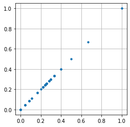
# Next, put the comparison through a quantitative litmus test.
np.allclose(reduced['loo_auto'].values, reduced['loo_manual'].values, atol=1)
# It fails the litmus test. There is disagreement that escaped eyeballing of the plot in the previous cell.False# First suspect: null values?
reduced.loc[reduced['loo_manual'].isnull(), 'cat5']
# Indeed, that's the culprit.108 BF
1083 BX
2223 CC
2329 AM
2956 BM
3827 R
4114 B
5235 J
6985 CG
8167 CB
8372 BJ
9533 BH
9687 P
Name: cat5, dtype: object# Next line of investigation: where do those null values originate from?
pblem_grp = reduced.loc[reduced['loo_manual'].isnull(), 'cat5'].values
reduced['cat5'].value_counts().loc[pblem_grp]
# They are from category groups which exist only on a single row.
# Our manual calculation was correct, because by definition it is not possible to encode Leave-One-Out for category groups with count=1.
# That's because by definition in Leave-One-Out encoding a given row leaves itself out, in this case it is left with no row.BF 1
BX 1
CC 1
AM 1
BM 1
R 1
B 1
J 1
CG 1
CB 1
BJ 1
BH 1
P 1
Name: cat5, dtype: int64# So how did LeaveOneOutEncoder get a non-null value?
reduced.loc[reduced['cat5'].isin(pblem_grp)][['target', 'loo_manual', 'loo_auto']]
# So LeaveOneOutEncoder plugs in as surrogate a constant value it found somewhere, 0.2626.# Let us make a wild guess where LeaveOneOutEncoder found the value 0.2626.
reduced['target'].mean()
# Voila.0.2626