Mutual information score
scikit-learn’s implementation, textbook algorithms and back-of-envelop calculations
explains why scikit’s results do not readily match our estimations
from sklearn import metrics, datasets
import numpy as np
import pandas as pd
import matplotlib.pyplot as plt
from matplotlib import cm
Example 1
# the next 5 lines for y and p are just to produce a cross tabulation containing
# unique values easy for demo purpose
y = [0] * 6
y.extend( [1] * 15)
y.extend( [2] * 24)
p = [0, 1, 1, 2, 2, 2, 0, 0, 0, 0, 1, 1, 1, 1, 1, 2, 2, 2, 2, 2, 2, 0,
     0, 0, 0, 0, 0, 0, 1, 1, 1, 1, 1, 1, 1, 1, 2, 2, 2, 2, 2, 2, 2, 2, 2]
df = pd.DataFrame(list(zip(y, p)), columns=['y', 'p'])
pd.crosstab(df.y, df.p, margins=True)
Loading...
Scikit-learn
metrics.mutual_info_score(y, p), metrics.normalized_mutual_info_score(y, p, average_method='arithmetic')(0.005463676561923342, 0.005316659245237883)Manual back-of-envelop calculation
MI = 1/45*np.log((1/45) / (12/45) / (6/45)) + 2/45*np.log((2/45) / (15/45) / (6/45)) + 3/45*np.log((3/45) / (18/45) / (6/45)) + \
     4/45*np.log((4/45) / (12/45) / (15/45)) + 5/45*np.log((5/45) / (15/45) / (15/45)) + 6/45*np.log((6/45) / (18/45) / (15/45)) + \
     7/45*np.log((7/45) / (12/45) / (24/45)) + 8/45*np.log((8/45) / (15/45) / (24/45)) + 9/45*np.log((9/45) / (18/45) / (24/45))
Hy = -6/45*np.log(6/45) -15/45*np.log(15/45) -24/45*np.log(24/45)
Hp = -12/45*np.log(12/45) -15/45*np.log(15/45) -18/45*np.log(18/45)
NMI = 2*MI/(Hy + Hp)
print(MI, NMI)
0.005463676561923696 0.005316659245238226
Putting back-of-envelop calculation into code
# implement algorithm according to
# https://scikit-learn.org/stable/modules/clustering.html
def calcmutualinfo0(df):
    ct = pd.crosstab(df.y, df.p, margins=True).values
    Hy, Hp, MI = 0, 0, 0
    for py in ct[:-1, -1]/ct[-1, -1]:
        Hy += -py * np.log(py)
    for pc in ct[-1, :-1]/ct[-1, -1]:
        Hp += -pc * np.log(pc)
    for col in range(ct.shape[1]-1):
        pc = ct[-1, col]/ct[-1, -1]
        for row in range(ct.shape[0]-1):
            py = ct[row, -1]/ct[-1, -1]
            pij = ct[row, col]/ct[-1, -1]
            if pij != 0:
                MI += pij * np.log(pij/pc/py)
    NMI = 2*MI/(Hy + Hp)
    print(MI, NMI)
calcmutualinfo0(df)
0.005463676561923696 0.005316659245238226
# implement algorithm like
# https://scikit-learn.org/stable/modules/clustering.html
# using log2 instead of log_natural
def calcmutualinfo1(df):
    ct = pd.crosstab(df.y, df.p, margins=True, normalize=True).values
    Hy, Hc, MI = 0, 0, 0
    for py in ct[:-1, -1]/ct[-1, -1]:
        Hy += -py * np.log2(py)
    for pc in ct[-1, :-1]/ct[-1, -1]:
        Hc += -pc * np.log2(pc)
    for col in range(ct.shape[1]-1):
        pc = ct[-1, col]
        for row in range(ct.shape[0]-1):
            py = ct[row, -1]
            pij = ct[row, col]
            if pij != 0:
                MI += pij * np.log2(pij/pc/py)
    NMI = 2*MI/(Hy + Hp)
    print(MI, NMI)
calcmutualinfo1(df)
0.007882419080908577 0.006344586884912296
# implement algorithm according to
# https://course.ccs.neu.edu/cs6140sp15/7_locality_cluster/Assignment-6/NMI.pdf
def calcmutualinfo2(df):
    ct = pd.crosstab(df.y, df.p, margins=True).values
    Hy, Hc, Hyc = 0, 0, 0
    for py in ct[:-1, -1]/ct[-1, -1]:
        Hy += -py * np.log2(py)
    for pc in ct[-1, :-1]/ct[-1, -1]:
        Hc += -pc * np.log2(pc)
    for col in range(ct.shape[1]-1):
        for row in range(ct.shape[0]-1):
            p = ct[row, col]/ct[-1, col]
            if p != 0:
                Hyc += -p * np.log2(p) * ct[-1, col]/ct[-1, -1]
    NMI = 2*MI/(Hy + Hp)
    print(MI, NMI)
calcmutualinfo2(df)
0.005463676561923696 0.004397732511094565
Example 2
np.random.seed(0)
n_samples = 1000
X, y = datasets.make_circles(n_samples=n_samples, factor=.5, noise=.01)
def plottis(X, y, p):
plt.set_cmap('Set1')
plt.scatter(X[:, 0], X[:, 1], c=p, s=3)
plt.axis('equal'); plt.axis('off')
plt.title('MI={:.1e}, NMI={:.1e}'.format(metrics.mutual_info_score(y, p), metrics.normalized_mutual_info_score(y, p, average_method='arithmetic')))plt.figure(figsize=(15, 15))
plt.subplot(331)
p = np.zeros(len(y))
p[X[:, 0]>-.6] = 1
plottis(X, y, p)
plt.subplot(332)
p = np.zeros(len(y))
p[X[:, 0]>-.9] = 1
plottis(X, y, p)
plt.subplot(333)
p = np.zeros(len(y))
p[X[:, 0]>0] = 1
plottis(X, y, p)
plt.subplot(334)
p = y.copy()
plottis(X, y, p)
plt.subplot(335)
p = np.zeros(len(y))
p[y==0] = 1
plottis(X, y, p)
plt.subplot(336)
X, y = datasets.make_circles(n_samples=n_samples, factor=.1, noise=.01)
p = y.copy()
plottis(X, y, p)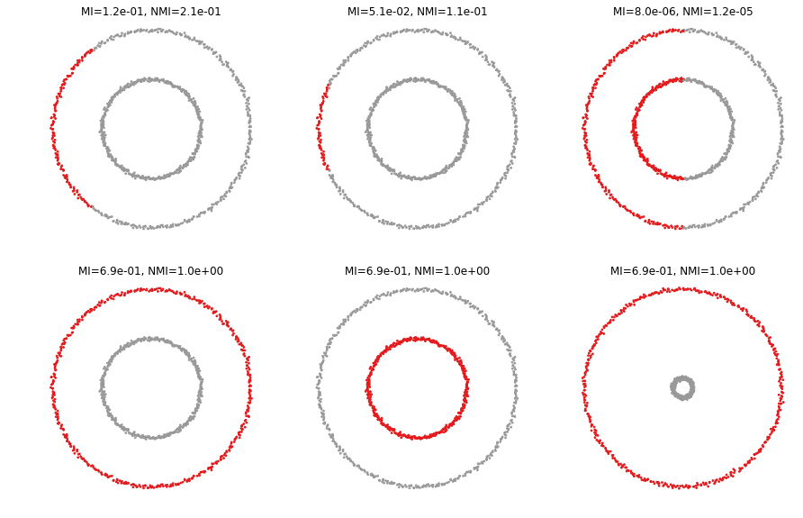
Example 3
plt.figure(figsize=(15, 7))
plt.subplot(131)
X, y = datasets.make_blobs(n_samples=n_samples, cluster_std=[1, 2.5, .5], random_state=77)
p = y.copy()
plottis(X, y, p)
plt.subplot(132)
p = y.copy()
p[(X[:, 0]>3) & (X[:, 0]<4)] = 0
plottis(X, y, p)
plt.subplot(133)
p = y.copy()
p[(X[:, 0]>3) & (X[:, 0]<4)] = 0
p[(X[:, 0]>8) & (X[:, 0]<10) & (X[:, 1]>2) & (X[:, 1]<4)] = 2
plottis(X, y, p)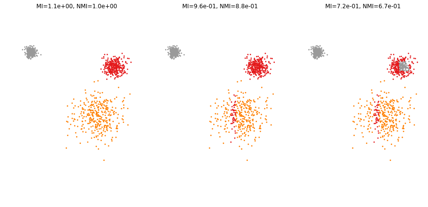
Example 4
centres = []
for i in np.arange(-50, 50, 10):
    for j in np.arange(-50 ,50, 10):
        centres.append([i, j])
X, y = datasets.make_blobs(n_samples=n_samples*100, centers=centres, random_state=77)
p = y.copy()
plt.figure(figsize=(15, 15))
plottis(X, y, p)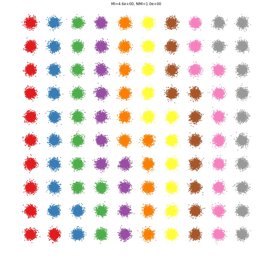
plt.figure(figsize=(15, 15))
p = y.copy()
# create an additional cluster and assign to it half of the points from each of the existing clusters
for i in range(100):
    j = np.where(p==i)[0][:500]
    p[j] = 1 + y.max()
    plt.plot(X[j, 0], X[j, 1], '.k', linewidth=.1)
plottis(X, y, p)